On Auxiliary Tasks in Deep Reinforcement Learning
In the world of reinforcement learning (RL), a newborn agent sometimes struggles at reaching goals that we wish it could achieve. RL practicers always augment it with auxiliary tasks, which help the agent to learn much faster, more robustly, and ideally perform better. In this post, I will summarize those auxiliary tasks used in deep RL, share ideas behind intuitions, and hopefully inspire you in related work.
Table of Contents
- What are Auxiliary Tasks?
- Enemy Detection
- Depth Prediction
- Loop Closure Classification
- Pixel Control
- Feature Control
- Reward Prediction
- Forward & Inverse Dynamics
- CPC|A
- Auxiliary Predictive Modeling Tasks
- Auxiliary Policies
- Summary
What are Auxiliary Tasks
It is uneasy to define Auxiliary Tasks in a nutshell because they are fairly different from each other. Some of them are task-specific, e.g., Enemy Detection, while some are generally applicable, e.g., Reward Prediction. Some of them are used to assist to learn better representations, e.g., Loop Closure Classification, while some are used to model relations between future and history context, e.g., CPC|A. Most of them can be implemented by optimizing explicit objective functions, while some can only be done by optimizing surrogate losses instead because the original objectives might be intractable, e.g., Auxiliary Predictive Modeling Tasks with ELBO. Some even build auxiliary policies with information asymmetry against the main policy and use them to regularize the main policy.
However, we can still find some common properties:
- They introduce additional losses, which are optimized jointly with the main RL objective, i.e., \(\mathbb{E}_\tau\left[\Sigma_t r\right(s_t, a_t\left) \right]\) or \(\mathbb{E}_\tau\left[\Sigma_t r\right(s_t, a_t\left) + \alpha \mathcal{H}\left( \pi\right)\right]\) in maximum entropy RL.
- They share parameters with the main neural network, introducing extra signals to update parameters and allowing, for example, better learning of representations and/or regularization of the main policy.
- They can be removed during inference, which adds no cost after your agents are deployed.
- They are self-supervised, meaning that you do not need to manually construct labels for training them.
So far, you may have a first glance at auxiliary tasks. Now let’s examine them one by one. I summarized several auxiliary tasks and listed them in chronological order (almost) by their appearance time. Hopefully, you will see how they evolved and became much more important for training RL agents.
Enemy Detection
The very first employment of auxiliary tasks in RL can be traced back to 2016 in the paper Playing FPS Games with Deep Reinforcement Learning, where authors augmented their models to exploit game features. Concretely, they trained a DRQN to play the game Doom by asking their models whether an enemy exists in the current frame. See the figure below for an illustration. This screenshot comes from here.
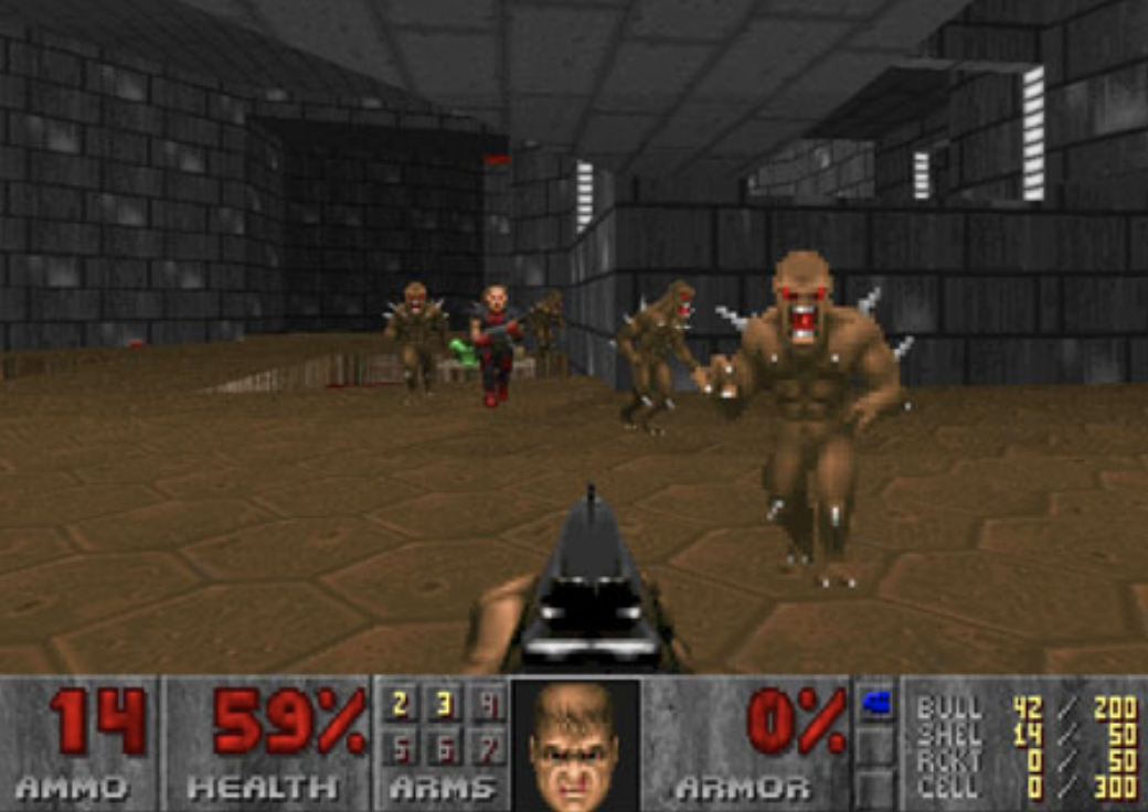
The motivation comes from the hypothesis that agents could not accurately detect enemies. To help them to better distinguish enemies appearing in the frame, at the output of CNN, they cascaded an MLP to answer the question about the appearance of enemies. Concretely, the MLP outputs the probability that enemies appear in the frame, which is then used to calculate a binary cross-entropy loss against binary labels provided by the game engine, i.e., \(\mathcal{L}_{EnemyDetection} = - \left(y_t\cdot \log P_t + (1 - y_t) \cdot \log (1 - P_t)\right)\). Pseudo-code is as below:
import torch

loss_enemy_detection = - torch.mean(label * torch.log(out_p) + (1 - label) * torch.log(1 - out_p))
Since gradients from this auxiliary loss can flow back to CNN, its parameters can be optimized toward more accurately capturing enemies, and hence provides the recurrent unit with information about the presence or absence of enemies, their locations, their distances, and so on. Authors reported doubled performance in terms of Kill-to-Death ratio of agents with enemy detection against those without.
As the first auxiliary task reported in RL literature, enemy detection is fairly intuitive and straightforward. In the original paper, the authors claim that one can build an MLP with k outputs to detect k game features, providing more possibility to improve the learning of representations. Notwithstanding, drawbacks are obvious. First, this design is quite task-specific and introduces extra requirements on the environment, i.e., your simulator should provide the relevant information you need. And also, detecting features in the current frame does not take account of temporal information. In my opinion, the auxiliary task of Reward Prediction that we will discuss later is a good alternative to Enemy Detection.
Depth Prediction
The auxiliary task of Depth Prediction is introduced in the paper Learning to Navigate in Complex Environments. It was proposed at almost the same time as Enemy Detection. The authors built an agent for navigation in complex 3D mazes, DeepMind Lab, and claimed higher data efficiency and task performance by jointly optimizing the RL objective and auxiliary losses of Depth Prediction and Loop Closure Classification (which we will discuss in the next section).
Depth maps reveal great information about 3D objects and 3D scenes. Grounding on the progress in CV, the auxiliary task of depth prediction asks agents to predict the depth information in the central field of view from multimodal sensory inputs, e.g., RGB observations, agent-relative velocity, etc. The depth predictor takes input either from convolutional layers or the LSTM. In the first case, the prediction only conditions on the current RGB observation, while in the latter case, the prediction conditions on the history of observations (RGB observation and agent-relative velocity), action, and reward, which is equivalent to condition the prediction on the belief state. From the view of POMDP, an agent cannot obtain the full state of the environment due to its partial observability \(O(\cdot \vert s,a)\). Therefore, to make decisions under uncertainty, the agent has to repeatedly ask itself the question “what is the real state I am currently at?”. Formally, we say the agent needs to maintain a distribution, \(P_b(\cdot \vert h_t)\), over true states given its history \(h_t = \{o_0, a_0, o_1, a_1, \ldots a_{t-1}, o_t\}\) and call this distribution belief state. You can understand this by thinking of the example of finding some location you’ve never visited without Google Map. You continuously update your guess about your current location by integrating what you’ve seen, e.g., buildings, landmarks, etc, and where you’ve moved. Now let’s get back to depth prediction. Intuitively, predicting the depth information given belief state is much easier than that solely given the current observation. What’s more, prediction conditioned on belief state also contributes gradients to the recurrent unit, helping to better model the representation of belief state and hence resulting in, ideally, higher task performance. Experimental results in the paper support this claim. Authors compared task performance of depth prediction conditioned on current RGB observation and belief state across four maps, i.e., small/large static/random mazes. I order these four maps by how partially observable they are: small static maze < large static maze < small random maze < large random maze. Agents trained using depth prediction conditioned on belief state outperform those conditioned on current RGB observation in all four maps. Furthermore, the superiority becomes more obvious as the map becomes more partially observable, i.e., 1.7% in the small static maze, 3.6% in the large static maze, 20.0% in the small random maze, and 28.8% in the large random maze. All agents augmented with depth prediction outperform their vanilla counterparts.
Now let’s see how it is implemented. First of all, considering the computational budget, the agent is asked to predict a cropped and subsampled depth map of size \(4 \times 16\), instead of the full-size map of \(84 \times 84\). An example of the prediction can be seen below. This screenshot is taken from the video released with the paper.
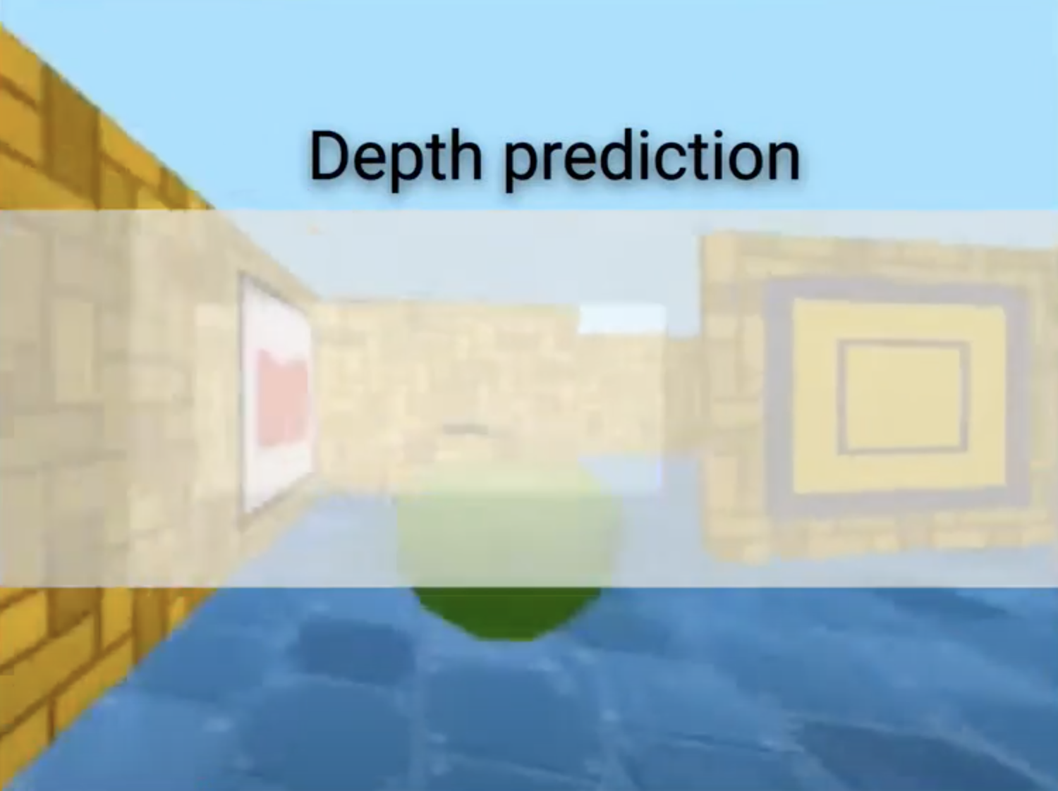
The prediction loss can be calculated in either a regression manner or a classification way. In the regression way, the loss for depth prediction at time step \(t\) can be computed as \(\mathcal{L}=\frac{1}{2} \Vert \hat{d}_t - d_t \Vert^2_2\). In the classification way, the depth value at each pixel is quantized into 8 intervals, which is subsequently used as labels with the predictor’s softmax outputs to calculate a cross-entropy loss. Specifically, the authors empirically used the non-uniformly quantization [0, 189, 214, 226, 234, 240, 245, 249, 255], which makes agents pay more attention to distant objects. Prediction as classification is reported better than that as regression. It is reasonable because prediction as classification softens the loss space to some extent and hence makes the learning easier.
Though the auxiliary task of depth prediction significantly speeds up learning navigation, Ye et al. argued that it is not generally applicable in both simulation and the real world and proposed to use more self-supervised tasks. Nevertheless, in my opinion, the idea of helping to represent belief states by predicting features of 3D objects/scenes from other modalities is much more valuable.
Loop Closure Classification
The auxiliary task of Loop Closure Classification is proposed with Depth Prediction in the same paper. The motivation is for the sake of more efficient exploration and spatial reasoning. Concretely, given locations up to time t in an episode ${p_0, p_1, \ldots , p_t}$, a loop closure label at time step t is true if $\vert p_t - p_j \vert \leq \eta_1$ where $j < t$ and $\vert p_t - p_{anchor}\vert \leq \eta_2$ where $p_{anchor}$ is an anchor point being far from $p_t$ to avoid trivial loops. An MLP works as the loop closure classifier conditioned on the hidden representation of the LSTM. This task is optimized by minimizing a binary cross-entropy loss between predictions and true labels.
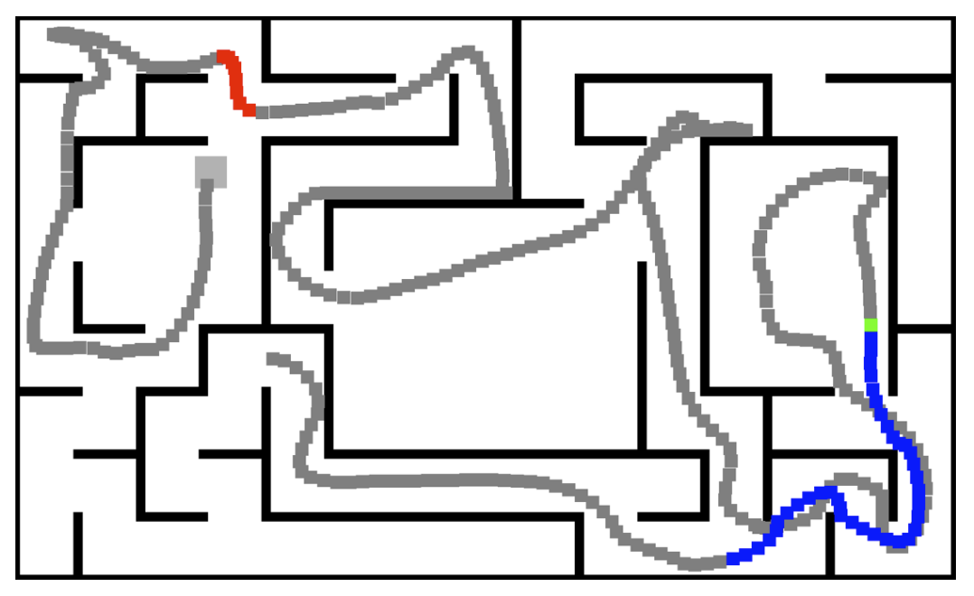
The following image is taken from Figure 4 in the original paper and shows a trajectory. The grey square represents the starting position. Grey dots show the paths of the agent. Blue dots represent true positive prediction (a loop closure happens and the classifier correctly predicts that). Red dots represent false-positive predictions. Green dots show false-negative predictions. It is interesting to note that the segment where the agent makes false positive predictions. The agent might reckon that it is in a loop only because it is close to the beginning. However, that segment is not in a loop during the exploration. This is one reason that I argue that this auxiliary task is a bit unnecessary and even detrimental to the task performance. Experimental results also support this argument that the task performance is not monotonically improved by augmenting with loop closure classification.
Pixel Control
Auxiliary tasks of Pixel Control, Feature Control, and Reward Prediction are proposed in the UNREAL agent. Motivated by the hypothesis that an agent can achieve any goals if it can control its future, the authors developed pixel control and feature control as auxiliary control tasks. To enable the agent to predict its future, they also proposed auxiliary reward tasks. All these tasks are unsupervised. Training them only relies on signals provided by pseudo reward functions, alleviating the reward sparsity generally encountered. Furthermore, policies for auxiliary tasks share parameters with the base policy, asking the agent to balance the main task and auxiliary tasks. We will talk about pixel control in this section by discussing its definition, motivation, and implementation. I also attached some Python codes for those who wish to implement it by themselves.
An auxiliary control task c is defined by a reward function \(r^{(c)}: \mathcal{S} \times \mathcal{A} \rightarrow \mathbb{R}\). Thinking of a baby crawling around in the garden, what he/she sees changes rapidly and dramatically to satisfy his/her curiosity. Likewise, the auxiliary task of pixel control is proposed to maximize the pixel changing in the perceptual stream. Concretely, using the averaged absolute pixel change between successive RGB observations as the reward signal, pixel control is optimized as an n-step Q-learning:
\[\mathcal{L}_{PC}^{(c)}= \mathbb{E}\left[ \left( R_{t:t+n} + \gamma^n \max_{a'} Q^{(c)} \left( s', a', \theta^{-}\right) - Q^{(c)}\left(s, a, \theta \right)\right) ^ 2 \right],\]where \(\theta^-\) represents parameters of the target Q function and the optimization is taken with respect to \(\theta\). The policy network for pixel control \(\pi^{(c)}\) takes the output from LSTM as input, enabling its access to the history of observations and rewards. The number of heads is equal to the number of action heads and each head outputs a $N_{act} \times n \times n$ Q-estimation.
In practice, visual observations are always cropped and subsampled. With a conventional size of $84 \times 84$ for image inputs, they are first cropped to the central $80 \times 80$ area and then subsampled with a factor of 4, resulting in the size of $20 \times 20$. The pseudo reward is computed as the average absolute pixel change between successive image observations, which is illustrated in the following code block.
import torch
import torch.nn.functional as F

# each side is cropped by 2
CROP = 2
# subsample factor
SSF = 4


def pixel_change_reward(observations):
    """
    Compute pixel change between successive RGB observations
    Args:
        observations (torch.Tensor): RGB observations of size (N, L + 1, C, H, W)
    Returns:
        pc_reward (torch.Tensor): Pseudo reward of size (N, L, H_crop_subsample, W_crop_subsample)
    """
    # crop obs
    observations = observations[:, :, :, CROP:-CROP, CROP:-CROP]
    # compute average absolute pixel change between successive images
    # (N, L + 1, C, H, W) -> (N, L, H, W)
    pixel_change = (observations[:, :-1] - observations[:, 1:]).abs().mean(2)
    # subsample
    # (N, L, H, W) -> (N, L, H / SSF, W / SSF)
    pc_reward = F.avg_pool2d(pixel_change, SSF, SSF)
    return pc_reward
A deconvolutional network, which exploits the spatial correlation, is used to produce $N_{act} \times 20 \times 20$ Q-estimation from the outputs of the LSTM. The dueling factorization is used to learn the value function more efficiently. Specifically, the deconvolutional network consists of two streams with 1 and $N_{act}$ output channels, producing the state value and advantage, respectively. Finally, with the pseudo reward we just calculated, the auxiliary task of pixel control can be optimized by minimizing the n-step Q-learning loss. Here is a code snippet demonstrating this process.
import torch
import torch.nn as nn


class PixelControl(object):
    """Compute the n-step Q learning loss for pixel control."""

    def __init__(self, model: nn.Module, gamma: float):
        """
        Args:
            model (nn.Module): your agent model with two attributes `pc_v` and `pc_adv`.
            gamma (float): discount factor
        """
        self._model = model
        self._gamma = gamma
        self._mse_loss = nn.MSELoss()

    def _calc_q(self, lstm_out: torch.Tensor, done: torch.Tensor):
        """
        Calculate Q values for pixel control.
        t-th done tells whether the t-th state is terminated
        Args:
            lstm_out (torch.Tensor): output from LSTM with shape (N, L + 1, hidden_size)
            done (torch.Tensor): (N, L + 1, 1)
        Returns:
            q_masked (torch.Tensor): q values with shape (N, L + 1, N_act, H, W)
        """
        # first we combine the first two axes
        lstm_out = lstm_out.reshape((-1, lstm_out.shape[-1]))
        # forward the v net
        v = self._model.pc_v(lstm_out)    # (N * (L + 1), 1, 20, 20)
        # forward the advantage net
        adv = self._model.pc_adv(lstm_out)    # (N * (L + 1), N_act, 20, 20)
        # now calculate q value with dueling factorization
        n_act = adv.shape[1]
        adv_mean = adv.mean(1, keepdim=True).repeat([1, n_act, 1, 1])
        q = v.repeat([1, n_act, 1, 1]) + adv - adv_mean    # (N * (L + 1), N_act, 20, 20)
        q = q.reshape((done.shape[0], done.shape[1], *q.shape[1:]))    # (N, L + 1, N_act, 20, 20)
        # now we need to mask q values for terminal states
        done = done.unsqueeze(-1).unsqueeze(-1).repeat([1, 1, *q.shape[2:]])
        q_masked = (1 - done) * q
        return q_masked

    def calc_loss(self, obs: torch.Tensor, lstm_out: torch.Tensor, action: torch.Tensor, done: torch.Tensor):
        """
        Calculate n-step Q loss for pixel control
        Args:
            obs (torch.Tensor): RGB observations of size (N, L + 1, C, H, W)
            lstm_out (torch.Tensor): output from LSTM with shape (N, L + 1, hidden_size)
            action (torch.Tensor): (N, L, 1)
            done (torch.Tensor): (N, L + 1, 1)
        Returns:
            Loss
        """
        # compute the pseudo reward
        r = pixel_change_reward(obs)    # (N, L, H_crop_subsample, W_crop_subsample)
        N, L = r.shape[0], r.shape[1]
        # mask r in terminal states
        mask = done[:, :-1]
        r = (1 - mask.unsqueeze(-1)) * r
        # compute q
        q = self._calc_q(lstm_out, done)    # (N, L + 1, N_act, H, W)

        # q estimations
        # we use a trick here to avoid loop
        q_estimate = q[:, :-1][
            torch.arange(N).unsqueeze(1).repeat([1, L]),
            torch.arange(L).unsqueeze(0).repeat([N, 1]),
            action.squeeze(-1)
        ]    # (N, L, H, W)
        # calculate q targets
        q_targets = []
        last_max_q = torch.max(q[:, -1:], dim=2).values
        temp = last_max_q
        for i in range(L - 1, -1, -1):
            temp = r[:, i:i + 1] + self._gamma * temp
            q_targets.append(temp)
        q_targets.reverse()
        # stop gradient for target
        q_targets = torch.cat(q_targets, dim=1).detach()    # (N, L, H, W)

        # finally calculate loss
        loss = self._mse_loss(q_estimate, q_targets)
        return loss
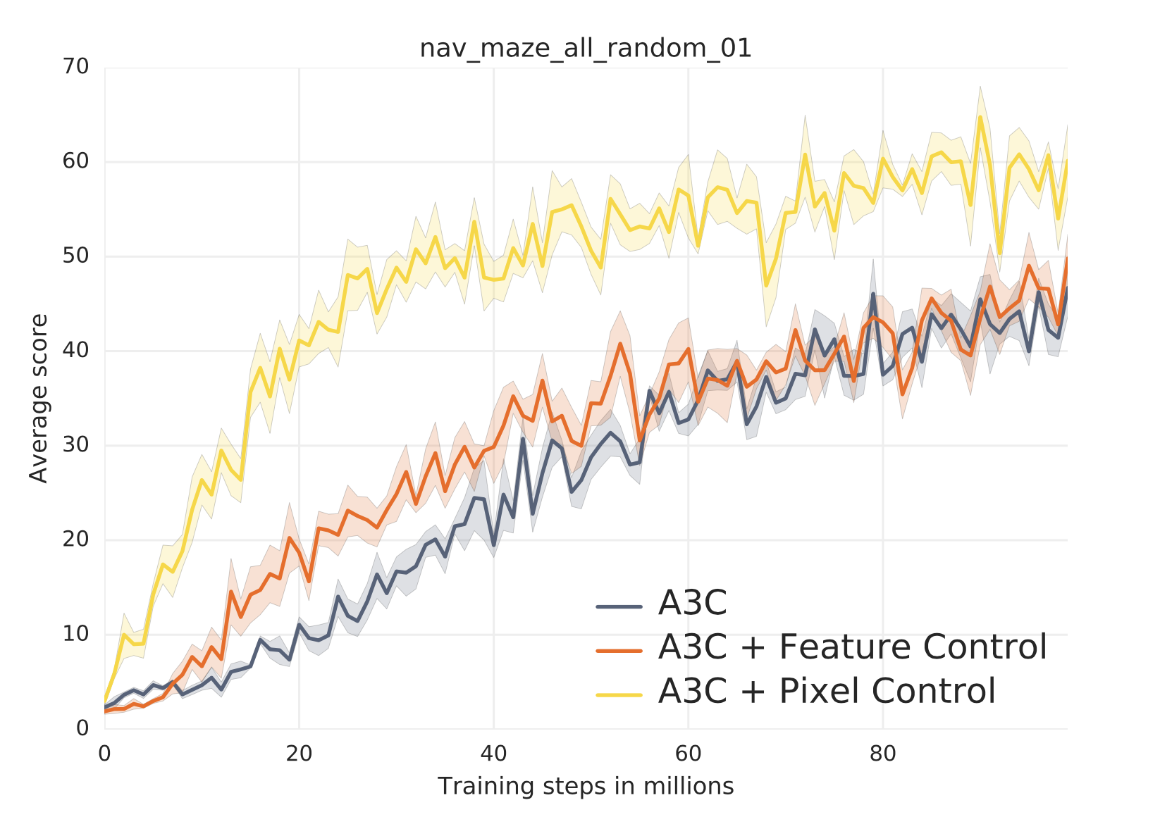
To find out how much the addition of pixel control helps the learning, let’s compare performances of a vanilla A3C agent, variants augmented with input reconstruction/input change prediction, and an A3C agent with pixel control. While the input reconstruction is optimized in a self-supervised manner with one head trying to reconstruct input images, the input change prediction is similar to pixel change instead of that it only predicts the auxiliary reward. The A3C agent with input reconstruction learns faster than the vanilla A3C agent at the beginning. However, it is worse than the vanilla one in terms of the final performance. Signals from input reconstruction loss speed up the learning of representation when training from scratch. However, the agent may struggle at reconstructing irrelevant features as the training continues, which instead limits its performance. Furthermore, the agent with input change prediction outperforms that with input reconstruction. My interpretation is that compared with only the current observation, change between successive observations takes into account some temporal information. Therefore, learning to predict the information is more beneficial for learning in such partially observable tasks. And hence, using an n-step Q learning loss to optimize the control of that information is much more beneficial due to the longer temporal dependencies involved, which leads to the best performance achieved by the agent with pixel control.
![]()
Feature Control
The auxiliary task of Feature Control is similar to pixel control, except that the quantity being controlled, i.e., feature, is expressed in a way that is much easier to understand for the neural networks. Concretely, activated outputs from hidden units are used as such quantity. The pseudo auxiliary reward is thus computed as the absolute difference between successive outputs from hidden units. In contrast to sensorimotor inputs such as RGB images, outputs from intermediate layers in the neural network consist of more high-level and more task-relevant information extracted by the model. That’s why I said that this auxiliary control task is learned in a more “model-friendly” way. To do so, we just need to replace the input to the previous function pixel_change_reward by, for example, outputs from the second convolutional layer of our CNN. The experiment shows that the A3C agent with feature control speeds up the learning from scratch, leading to higher data efficiency.
Reward Prediction
A good agent should be able to recognize states leading to high reward and value. However, learning of such recognization is challenging in many environments due to reward sparsity. The auxiliary task of Reward Prediction with a specially designed experience replay buffer aims to mitigate this issue without introducing any bias into the agent’s policy. It asks the agent to predict the immediate reward given some history of observations. Since gradients from such supervised signals do not flow back to the policy network, it only helps to shape the features and does not bias policy or value. To be specific, the agent is given a history of embedded observations \(H_{\tau}=\{f\left(o_{\tau - k}\right),f\left(o_{\tau - k+1}\right),\ldots,f\left(o_{\tau - 1}\right)\}\) and asked to predict the immediate reward \(r_\tau\) in the subsequent unseen frame. This is equivalent to a myopic version of TD(1), i.e., \(\gamma=0\):
\[\begin{align} \mathcal{L}_{RP} &=\mathbb{E}_{H_\tau \sim \mathcal{H}} \left[\left( r_\tau + \gamma f_{RP}\left(H_{\tau+1}; \phi_{RP}\right) - f_{RP}\left(H_\tau;\phi_{RP}\right) \right)^2\right] \bigg\rvert_{\gamma=0} \\ &=\mathbb{E}_{H_\tau \sim \mathcal{H}} \left[\left( r_\tau - f_{RP}\left(H_\tau;\phi_{RP}\right) \right)^2\right] , \end{align}\]where \(f_{RP}\left(\cdot; \phi_{RP}\right)\) is the network parameterized by\(\phi_{RP}\) predicting the reward and \(\mathcal{H}\) is a specially designed experience replay buffer for this auxiliary task, which I shall explain later. In practice, it is trained by minimizing a cross-entropy loss with three classes, i.e., zero-reward class, positive-reward class, and negative-reward class.
To overcome the reward sparsity, an experience replay buffer is intentionally split to be two parts, one for zero-reward histories and the other for rewarding histories. Samples are equally replayed from these two subsets such that \(P\left(r_\tau \neq 0\right) = 0.5\). This replay buffer is demonstrated in the figure below.
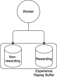
We use a length of 3 for context in experiments and the following code snippet. To simplify the temporal dependencies and only ask the agent to focus on predicting the immediate reward, the computation is done in a feedforward manner. An MLP is used to predict the label from stacked 3 successive embedded features from CNN. Gradients from the cross-entropy loss between predictions and ground truths thus help to shape and speed up the learning of features. I demonstrate this process in the code block below.
from collections import deque

import numpy as np
import torch
import torch.nn as nn


class Worker(object):
    """A simple worker that interacts with env and generates samples"""

    def __init__(self, history_len: int = 3):
        """
        Args:
            history_len (int): length of history context for reward prediction
        """
        # we use a deque to cache history context
        self._cache = deque(maxlen=history_len + 1)
        self._hist_len = history_len

    def rollout(self):
        # initialize an env
        env = Env()

        # reset env
        obs, reward, done, info = env.reset()
        # add obs to cache
        self._cache.append(obs)

        # start rollout
        done = False
        while not done:
            action = self._act(obs)
            obs, reward, done, info = env.step(action)
            # add obs to cache
            self._cache.append(obs)
            # push history context
            if len(self._cache) >= self._hist_len + 1:
                history_context = np.array(
                    [self._cache.popleft() for _ in range(self._hist_len)]
                )
                # now push history context to corresponding replay buffer according to the immediate reward
                if reward == 0:
                    self._push_to_non_rewarding_replay(
                        {
                            'history_context': history_context,
                            'rp_label': np.array([1, 0, 0])
                        }
                    )
                else:
                    self._push_to_rewarding_replay(
                        {
                            'history_context': history_context,
                            'rp_label': np.array([0, 1, 0]) if reward > 0 else np.array([0, 0, 1])
                        }
                    )


class RewardPrediction(object):
    """Compute the cross entropy loss for reward prediction."""

    def __init__(self, model: nn.Module):
        """
        Args:
            model (nn.Module): your agent model with attribute `rp_mlp` and `cnn`
        """
        self._model = model

    def calc_loss(self, history: torch.Tensor, label: torch.Tensor):
        """
        Args:
            history (torch.Tensor): history context of RGB observations with shape (N, hist_len, C, H, W)
            label (torch.Tensor): labels for reward prediction with shape (N, 3)
        """
        # first we combine the first two axes
        N, HIST_LEN, C, H, W = history.shape
        history = history.reshape((N * HIST_LEN, C, H, W))

        # we call the CNN to process these history contexts
        # we assume your CNN outputs flattened features
        extracted_history = self._model.cnn(history)    # (N * HIST_LEN, -1)

        # we recover the dimension for history length
        extracted_history = extracted_history.reshape((N, HIST_LEN, -1))    # (N, HIST_LEN, -1)
        # we stack successive observations
        extracted_history = extracted_history.reshape((N, -1))    # (N, -1)

        # now we feed those features to the reward prediction MLP to get logits
        logits = self._model.rp_mlp(extracted_history)    # (N, 3)
        # we softmax the logits to get predicted probabilities
        prob = torch.softmax(logits, dim=-1)    # (N, 3)
        # we compute the cross entropy loss
        loss = -torch.sum(label * torch.log(prob), dim=1).mean()
        return loss
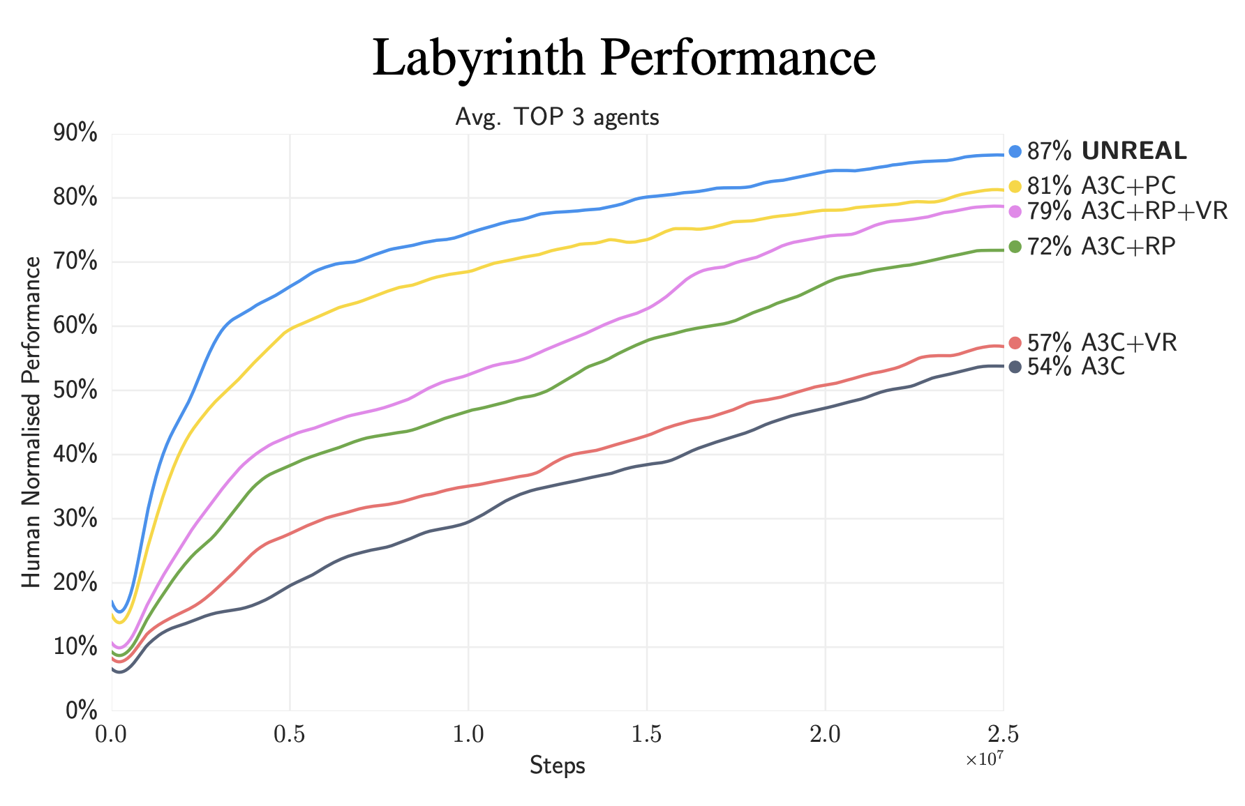
To see the performance gain brought by reward prediction, let’s compare a vanilla A3C agent and one augmented with reward prediction on a series of maze tasks in DM Lab. The augmented agent significantly outperforms the vanilla one by 33%. In my experience, for agents, the task of reward prediction in DM Lab tasks is fairly easy to learn because the semantic information is quite straightforward. For instance, an agent can predict positive when it sees a green and round object (an Apple in DM Lab, which is worth +1 reward) or an orange and stacked object (the Goal in DM Lab, which is worth +10 reward) and predict negative when it sees a yellow and round object (a Lemon, which is -1 reward). Thus agents learn the representation of features similar to learn object detection. However, in environments where semantic information relating to rewards is much more complicated and abstract, the performance on this auxiliary task degrades and becomes harder to converge. A simple way to verify this phenomenon is to replace the RGB observation, from which the reward label is predicted, with depth observation in which rewarding objects should be learned through their shapes instead of colors. Therefore, I reckon that although this auxiliary task is generally applicable, the difficulty of learning it and the performance gain it can bring may depend on environment complexity and the modality of sensorimotor inputs.
Forward & Inverse Dynamics
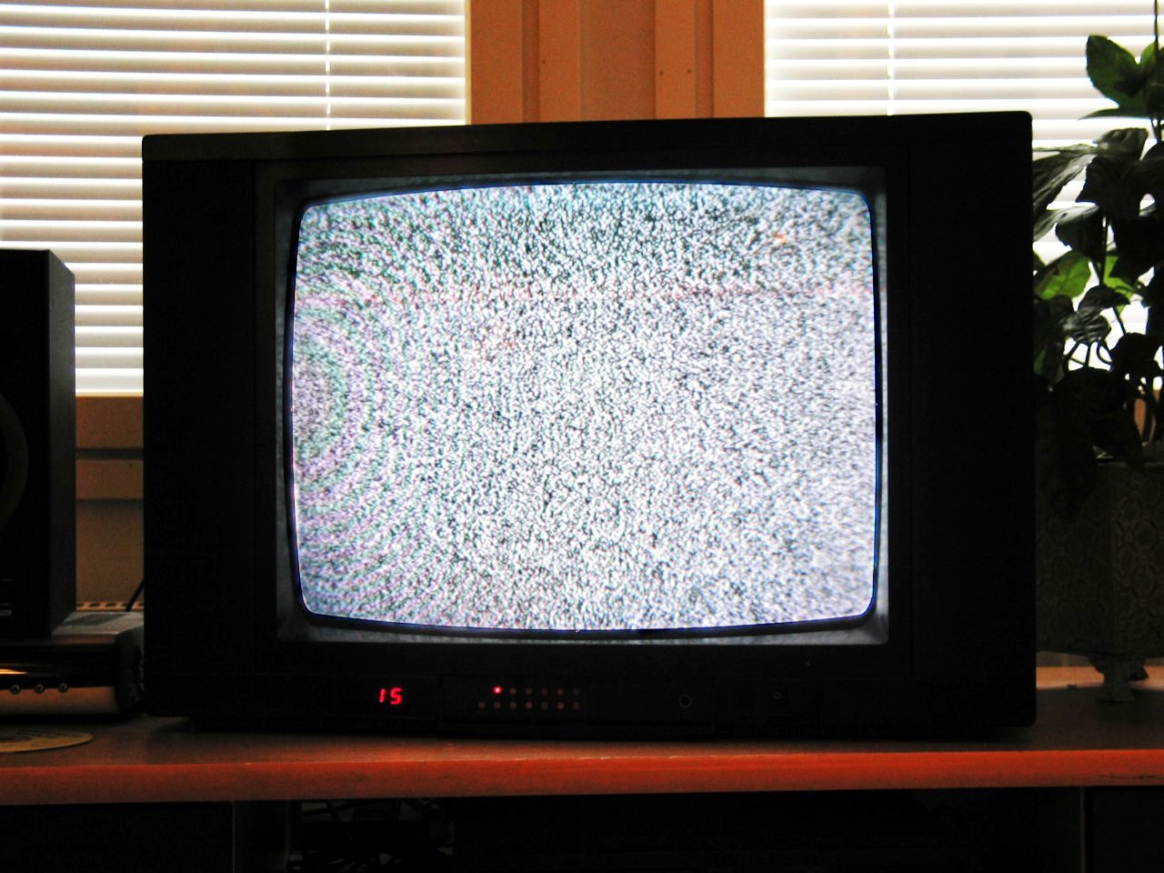
Generating intrinsic reward signals is a way in RL to help agents explore more novel states and to encourage them to perform actions that can reduce uncertainties in their belief states. In 2017, Pathak et al. proposed to use curiosity as an intrinsic signal which they defined as the error of the agent’s prediction of the consequences of its actions. To avoid falling into an artificial curiosity trap, an agent should embed observations into a feature space where only takes into account things under its control or things that can affect it (imagining that there is a television showing random Gaussian noise, an agent rewarded by its prediction discrepancy but cannot distinguish task-irrelevant variations will do nothing but watch that TV forever). A forward dynamics model and an inverse dynamics model are proposed to learn that feature space. Their corresponding proxy objectives and the main RL object are jointly optimized during training. A forward dynamics model \(f(\cdot;\theta_F)\) is a predicator of the feature representation of the next observation \(\phi(o_{t+1})\) given the feature representation of the current observation \(\phi(o_t)\) and the action taken \(a_t\). To build such a model, an agent should have enough knowledge about the underlying environments in a learnable embedded space. But how can it learn such a space that only embeds task-relevant information and features that can be controlled by itself? The inverse dynamics model provides extra self-supervised signals to do that. An inverse dynamics model \(g(\cdot ; \theta_I)\) takes representations of successive observations \(\phi(o_t)\) and \(\phi(o_{t+1})\) and tries to tell which action \(\hat{a_t}\) causes that transition. By concurrently training these two models, the encoder \(\phi(\cdot):\mathcal{O} \rightarrow \mathcal{F}\) will be good enough at neglecting task-irrelevant and uncontrollable variations and encoding from observation space \(\mathcal{O}\) to feature space \(\mathcal{F}\) in which the agent can predict consequences of its actions.
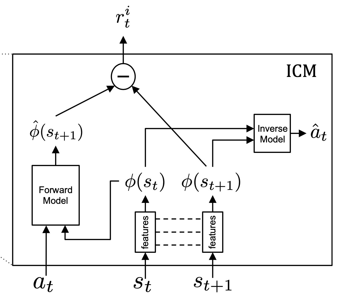
Now let’s look at the forward and inverse dynamics models and auxiliary tasks alongside them in more detail. The diagram below, which is from the original paper of Pathak et al., shows how they work. The observation at time step \(t\) is RGB or RGBD image. At each time step, the forward dynamics model predicts the feature representation of the next observation. The discrepancy between the prediction and the true feature representation of the successive observation is used as an intrinsic bonus awarded to the agent, i.e., \(r_t^i=\eta \left\Vert \hat{\phi}(s_{t+1}) - \phi(s_{t+1}) \right\Vert_2^2\), where \(\hat{\phi}(s_{t+1}) = f\left(\phi(s_t), a_t;\theta_F \right)\). Parameters of the forward dynamics model are optimized by minimizing the MSE loss:
\[\theta_F = \mathop{\mathrm{arg\,min}}_{\theta_F} \frac{1}{2} \left\Vert f\left(\phi(s_t), a_t;\theta_F \right) - \phi(s_{t+1}) \right\Vert^2_2.\]The inverse dynamics model is fed with feature representations of successive observations and tries to predict the action causing that transition, i.e., \(\hat{a}_t = g\left(\phi\left(s_t \right), \phi \left(s_{t+1}\right); \theta_I \right)\). Parameters \(\theta_I\) is optimized in a maximum-likelihood manner under multinomial distributions:
\[\theta_I = \mathop{\mathrm{arg\,min}}_{\theta_I} \sum^{\left\vert\mathcal{A} \right\vert}_i -a_t^{(i)} \cdot \log P_t^{(i)},\]where \(a_t^{(i)}\) and \(P_t^{(i)}\) is the indicator of the \(i\)-th action entry and predicted probability of that action at time step \(t\), respectively.
In the code demo below, we assume that the encoder \(\phi\) is a typical CNN which outputs flattened features and that forward and inverse models are MLPs. The forward MLP firstly concatenates the embedded observation at time step \(t\) with one-hot encoded action sampled from policy and then outputs a vector with the same size as the embedded observation. The inverse dynamics model takes input from concatenated vectors of embedded successive observations and outputs logits used to produce a categorical distribution of actions.
import torch
import torch.nn as nn


class ICM(object):
    """
    Intrinsic Curiosity Module in Curiosity-driven Exploration by Self-supervised Prediction, Pathak et al., ICML 2017
    https://arxiv.org/abs/1705.05363
    """

    def __init__(self, model: nn.Module):
        """
        Args:
            model (nn.Module): neural network model which has attributes `encoder`, `forward_dyn`, and `inverse_dyn`.
        """
        self._model = model
        self._mse_loss = nn.MSELoss()
        self._nll_loss = nn.NLLLoss()
        self._log_softmax = nn.LogSoftmax(dim=1)

    def forward_dynamics_loss(self, obs: torch.Tensor, action: torch.Tensor):
        """
        Args:
            obs (torch.Tensor): image observations with shape (N, L + 1, C, H, W)
            action (torch.Tensor): one-hot encoded actions with shape (N, L, A), where A is the number of actions
        """
        # first we combine N & L axes
        N, L = action.shape[0], action.shape[1]
        obs = obs.reshape((N * (L + 1), *obs.shape[2:]))    # (N, L + 1, C, H, W) -> (N * (L + 1), C, H, W)

        obs_emb = self._model.encoder(obs)    # (N * (L + 1), -1)
        # recover N & L axes
        obs_emb = obs_emb.reshape((N, L + 1, -1))    # (N * (L + 1), -1) -> (N, L + 1, emb_size)

        # concatenate obs_emb with one-hot encoded action as input to forward dynamics model
        emb_obs_with_action = torch.cat([obs_emb[:, :-1], action], dim=-1)    # (N, L, 1 + emb_size)
        # predict embedding of the next obs
        pred_emb_obs = self._model.forward_dyn(emb_obs_with_action)    # (N, L, emb_size)
        # compute the forward dynamics loss
        loss = self._mse_loss(pred_emb_obs, obs_emb[:, 1:])
        return loss

    def inverse_dynamics_loss(self, obs: torch.Tensor, action: torch.Tensor):
        """
        Args:
            obs (torch.Tensor): image observations with shape (N, L + 1, C, H, W)
            action (torch.Tensor): one-hot encoded actions with shape (N, L, A), where A is the number of actions
        """
        # first we combine N & L axes
        N, L = action.shape[0], action.shape[1]
        obs = obs.reshape((N * (L + 1), *obs.shape[2:]))    # (N, L + 1, C, H, W) -> (N * (L + 1), C, H, W)

        obs_emb = self._model.encoder(obs)    # (N * (L + 1), -1)
        # recover N & L axes
        obs_emb = obs_emb.reshape((N, L + 1, -1))    # (N * (L + 1), -1) -> (N, L + 1, emb_size)

        # concatenate successive obs_emb
        suc_obs_emb = torch.cat([obs_emb[:, :-1], obs_emb[:, 1:]], dim=-1)    # (N, L, 2 * emb_size)
        # compute logits
        logits = self._model.inverse_dyn(suc_obs_emb)    # (N, L, A)
        # compute cross entropy loss
        loss = self._nll_loss(
            self._log_softmax(logits.reshape((N * L, -1))),     # log prob
            torch.argmax(action.reshape((N * L, -1)), dim=1)    # target
        )
        return loss
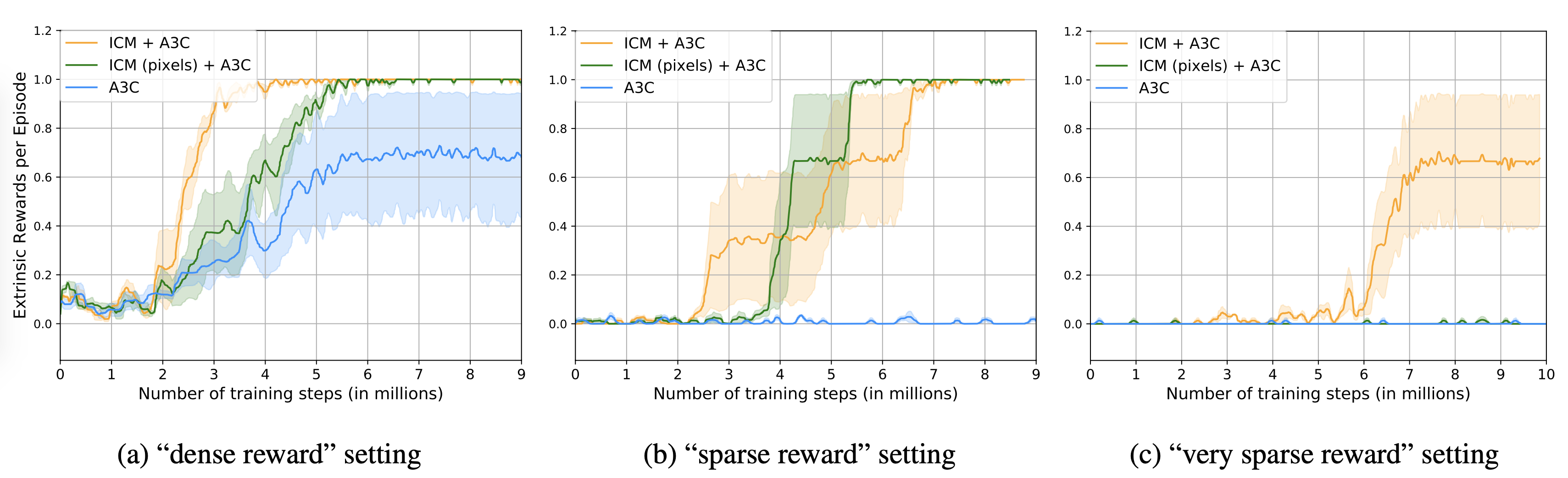
Now let’s see the comparison results between an A3C agent augmented with these two auxiliary tasks, one variant only augmented with forward dynamics model, and a vanilla A3C agent. The one only with forward dynamics model predicts observations in pixel space and uses prediction errors as an intrinsic reward. It shows that the full agent (ICM + A3C) achieves the best performance and enjoys the fastest learning speed in all settings with different sparsity of extrinsic reward. Furthermore, in the hardest setting, i.e., a very sparse reward setting, only the full agent can solve the task. The one predicting states in pixel space, i.e., ICM (pixels) + A3C, fails potentially due to the increased complexity of visual textures or even due to the unclarity of the effectiveness of predicting pixels as the objective. This is similar to the phenomenon that happened in pixel control we just discussed where an agent augmented with input reconstruction performs badly.
CPC|A
Contrastive Predictive Coding (CPC) is an unsupervised learning approach used to extract representations from high-dimensional data such as images. Instead of modeling a generative model \(p_k\left(x_{t+k} \vert c_t\right)\) between future observations \(x_{t+k}\) and context \(c_t\), it models a density ratio function \(f_k \left(x_{t+k}, c_t\right) \propto \frac{p_k\left(x_{t+k} \vert c_t\right)}{p_k\left(x_{t+k} \right)}\) by maximizing the mutual information between \(x_{t+k}\) and \(c_t\), i.e.,
\[\begin{align} I\left(x_{t+k};c_t \right) &= \sum_{x_{t+k}, c_t} p_k \left(x_{t+k},c_t \right) \log \frac{p_k \left(x_{t+k} , c_t \right)}{p_k \left(x_{t+k} \right) p_k \left(c_t\right)} \\ &=\sum_{x_{t+k}, c_t} p_k \left(x_{t+k},c_t \right) \log \frac{p_k \left(x_{t+k} \vert c_t \right)}{p_k \left(x_{t+k} \right)}. \end{align}\]This is achieved by minimizing a loss function based on NCE, named as InfoNCE:
\[\mathcal{L}_N = - \mathbb{E}_X \left[\log \frac{f_k \left(x_{t+k}, c_t\right)}{\sum_{x_j \in X}f_k \left(x_j, c_t \right)} \right].\]Intuitively, minimizing this loss leads to the probability begin maximized of classifying a positive sample from the conditional distribution \(p_k\left(x_{t+k} \vert c_t\right)\).
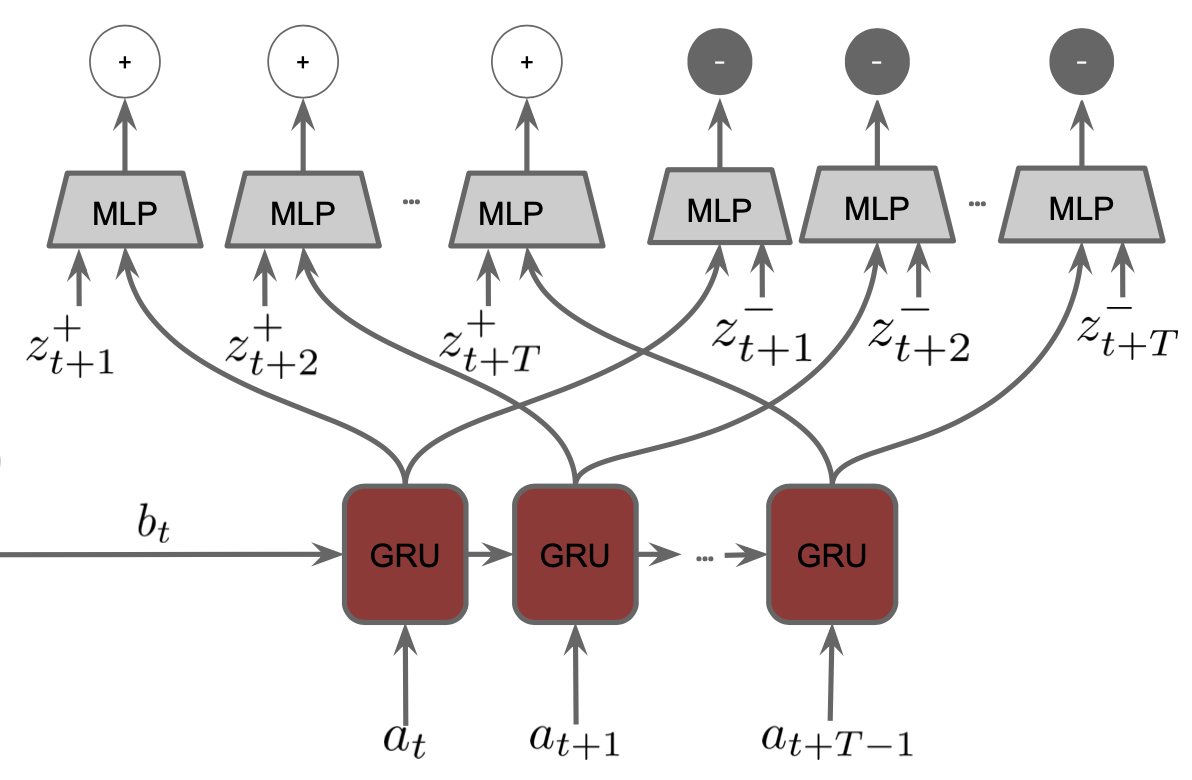
CPC|A (CPC conditioned on actions) is proposed by Guo et al. in 2018. When implementing CPC, practicers can use an autoregressive model such as LSTM and GRU as the density ratio function \(f_k \left(x_{t+k}, c_t\right)\). Similarly, the density ratio function in CPC|A can also be implemented using an RNN, except that future actions are fed to it. Concretely, at time step \(t\), the CPC|A GRU is initialized with the hidden state \(b_t\) of a belief module (e.g., an LSTM) which summarizes histories of observations and actions. Then, it is unrolled for \(T\) steps and fed by a series of future actions \(\{a_{t+i}\}_{i=0}^{T-1}\). Outputs at each future step are concatenated with either an embedding of positive observations (e.g., the RGB image observed at that time step) or an embedding of negative observations (e.g., RGB images randomly drawn from a buffer). An MLP classifier is asked to predict 1 for positive embeddings and 0 for negative embeddings. The diagram below, which is taken from Guo et al., gives an illustration.
I implement CPC|A in the following code block with reference to this repo.
import torch
import torch.nn as nn


class ActionConditionedCPC(nn.Module):
    """
    Implementation of CPC|A.
    https://arxiv.org/abs/1811.06407
    """
    def __init__(
        self,
        gru_hidden_size: int,
        gru_input_size: int,
        mlp_hidden_size: int,
        feature_size: int,
        k: int,
    ):
        """
        Args:
            gru_hidden_size (int): hidden size of CPC|A GRU.
            gru_input_size (int): input size of CPC|A GRU.
            mlp_hidden_size (int): hidden size of the MLP classifier.
            feature_size (int): output size of the feature encoder (e.g., CNN).
            k (int): predict k steps in the future.
        """
        super(ActionConditionedCPC, self).__init__()
        # create CPC|A GRU
        self._gru_cpca = nn.GRU(
            input_size=gru_input_size,
            hidden_size=gru_hidden_size,
        )
        # create an MLP classifier
        self._classifier = nn.Sequential(
            nn.Linear(feature_size + gru_hidden_size, mlp_hidden_size),
            nn.ReLU(),
            nn.Linear(mlp_hidden_size, 2)
        )

        self._k = k

        self._cross_entropy_loss = nn.CrossEntropyLoss()

    def compute_loss(
        self,
        obs_emb: torch.Tensor,
        act_emb: torch.Tensor,
        init_hidden_state: torch.Tensor,
    ):
        """
        Args:
            obs_emb (torch.Tensor): embeddings of future observations with shape (N, L + 1, feature_size) where L >= k.
            act_emb (torch.Tensor): embeddings of future actions with shape (N, L, gru_input_size) where L >= k.
            init_hidden_state (torch.Tensor): hidden state used to initialize CPC|A GRU with shape (N, gru_hideen_size)
        """
        N, L = act_emb.shape[0], act_emb.shape[1]
        assert L >= self._k

        # positive embeddings are those of real obs at future time steps
        # obs_emb[:, 0] is the embedding of obs at time step t
        # so we start from 1 for embedding of future obs
        pos_emb = obs_emb[:, 1:]

        # negative embeddings are embeddings of obs not at those time steps
        # they can be drawn from a buffer
        # but here we use permuted positive embeddings
        perm_idx = torch.randperm(N * L, device=obs_emb.device).unsqueeze(-1)
        neg_emb = torch.gather(
            obs_emb[:, 1:].reshape((N * L, -1)),
            dim=0,
            index=perm_idx.repeat([1, obs_emb.shape[-1]])
        )
        neg_emb = neg_emb.reshape((N, L, -1))

        # now we ask the GRU to unroll k-steps into the future
        act_emb = act_emb[:, :self._k]    # (N, K, -1)
        gru_out, _ = self._gru_cpca(
            act_emb.permute(1, 0, 2),
            init_hidden_state.unsqueeze(0),
        )
        gru_out = gru_out.permute(1, 0, 2)    # (K, N, -1) -> (N, K, -1)

        # assemble inputs for the MLP classifier
        pos_inputs = torch.cat([pos_emb, gru_out], dim=-1)    # (N, K, feature_size + gru_hidden_size)
        neg_inputs = torch.cat([neg_emb, gru_out], dim=-1)    # (N, K, feature_size + gru_hidden_size)
        # combine N & K axes
        pos_inputs = pos_inputs.reshape((-1, pos_inputs.shape[-1]))
        neg_inputs = neg_inputs.reshape((-1, neg_inputs.shape[-1]))

        # get logits from the MLP classifier
        pos_logits = self._classifier(pos_inputs)    # (N * K, 2)
        neg_logits = self._classifier(neg_inputs)    # (N * K, 2)

        # get loss
        pos_loss = self._cross_entropy_loss(
            pos_logits,
            torch.ones_like(pos_logits).long()[:, 0]
        )
        neg_loss = self._cross_entropy_loss(
            neg_logits,
            torch.zeros_like(neg_logits).long()[:, 0]
        )
        return pos_loss + neg_loss
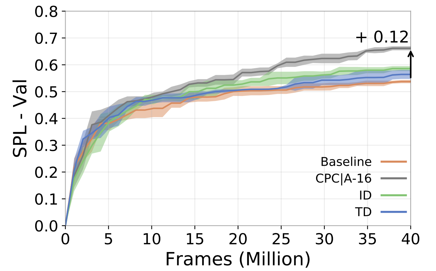
Ye et al. claimed an improvement of 0.12 SPL (Success weighted by Path Length) for task PointNavigation in Habitat by augmenting CPC|A-16 (predicting 16 future steps) over a DD-PPO baseline. The augmented agent enjoys higher data efficiency as well. The figure below is taken from Ye et al. to demonstrate the improvement brought by CPC|A.
Auxiliary Predictive Modeling Tasks
A human can encode, consolidate, and store streams of sensorimotor inputs (e.g., what you see, what you hear, what you touch, what you taste, etc.) and retrieve this stored information for predictions of upcoming events. For example, once you tried a dish with an impressive taste. Next time you see it, you probably will recall that taste. Neuroscientists found that the hippocampus in brains participates in the encoding, consolidation, and retrieval of memories. Similarly, in the world of RL, memory is necessary for agents to tackle partial observability in raw sensory data. With the idea of predictive modeling, Wayne et al. proposed a memory-based predictor (MBP) which compresses and stores observations and retrieves a series of history observations to make predictions. Similar to model the marginal distribution \(\log p \left( x\right)\), the MBP is trained toward predicting consistently with the probabilities of observed sensorimotor streams from the environment. Sadly, this objective is intractable to be optimized. Nevertheless, the surrogate objective ELBO can be used for the optimization of MBP. As we know that ELBO consists of two terms, one is the reconstruction loss and the other serves as a regularization against the complexity of the variational posterior. When exposing steams with multiple modalities, e.g., images, text instructions, velocities, the reconstruction loss can be a combination of all of them. These reconstruction tasks can be considered as auxiliary reconstruction tasks of additional heads trained under individual reconstruction loss.
Considering training RL agents in DM Lab as in Wayne et al., they get text instructions, observe images, and know their last action and corresponding reward. Some extra information about their dynamics such as velocity is also available. The MBP is trained via optimizing ELBO such that distributions of these observations can be modeled. Specifically, we build an image decoder, a return prediction decoder, a text decoder, a reward decoder, a velocity decoder, and an action decoder. Input to these decoders is one realization from the posterior distribution \(z_t \sim \mathcal{N}\left(\mu_t^q, \Sigma_t^q\right)\). Each decoder tries to reconstruct the observation in its corresponding modality. Assuming independence between these loss terms, the negative conditional log-likelihood can be expressed as
\[\begin{align} -\log p \left(o_t, R_t \vert z_t \right) &\equiv \alpha_{image} \mathcal{L}_{image} + \alpha_{return}\mathcal{L}_{return} + \alpha_{reward}\mathcal{L}_{reward}\\ &+ \alpha_{action}\mathcal{L}_{action} + \alpha_{velocity}\mathcal{L}_{velocity} + \alpha_{text} \mathcal{L}_{text}. \end{align}\]Besides reconstruction losses, the variational posterior is also regularized to the prior distribution through KL divergence \(D_{KL} \left(\mathcal{N}\left(\mu_t^q, \Sigma_t^q\right)\Vert \mathcal{N} \left(\mu_t^p, \Sigma_t^p\right) \right)\), resulting in a lower bound to the MBP loss:
\[\mathcal{L}_t \geq \mathbb{E}_{z_{\tau} \sim \mathbb{Q}_t} \left[\log p \left( o_{\tau}, R_\tau \vert z_\tau \right) - D_{KL} \left(\mathbb{Q}_t, \Vert \mathbb{P}_t \right)\right].\]Next, let’s see one comparison between an agent augmented with predictive modeling (MERLIN) and two baseline agents. This result is from Wayne et al., where the solid orange line represents MERLIN, the blue represents an RL-LSTM agent, the pink represents an RL-MEM agent, and the dotted orange shows the negative ELBO.
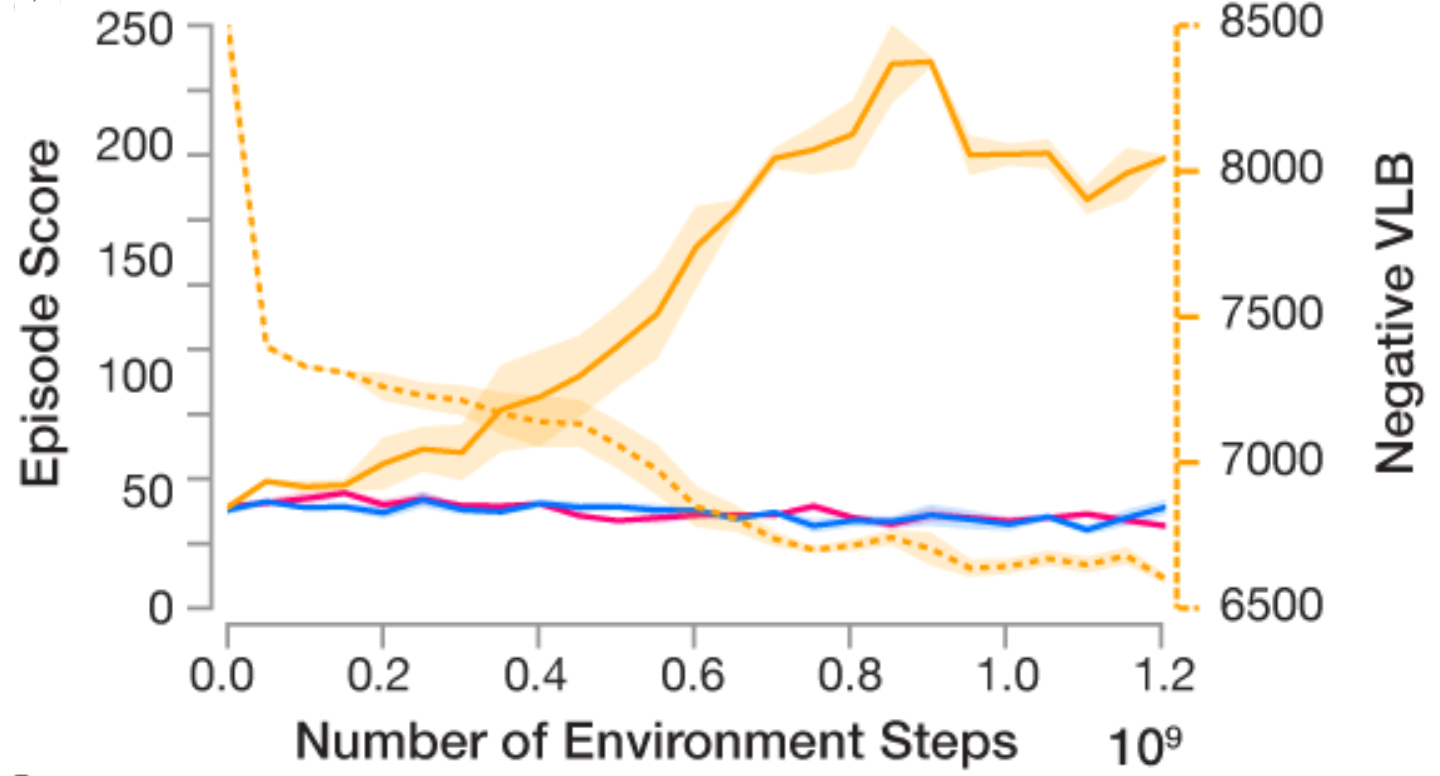
This task is Watermaze which tests the memory ability of agents. As we can see as the training goes on, the episode score increases while the negative VLB (variational lower bound, same as ELBO) decreases. The positive correlation between the performance and ELBO suggests that as the MBP can model and predict sensorimotor steams more accurately, the agent can do better in the memory task. The more goal-directed behavior in turn facilitates the learning of the MDP as the agent is more likely to be exposed to upcoming streams whose distributions are becoming more and more predictable (i.e., the ongoing observations will become more correlated to positive rewards). By contrast, two baseline agents fail to solve this task.
More details about MERLIN will be discussed in a future post.
Auxiliary Policies
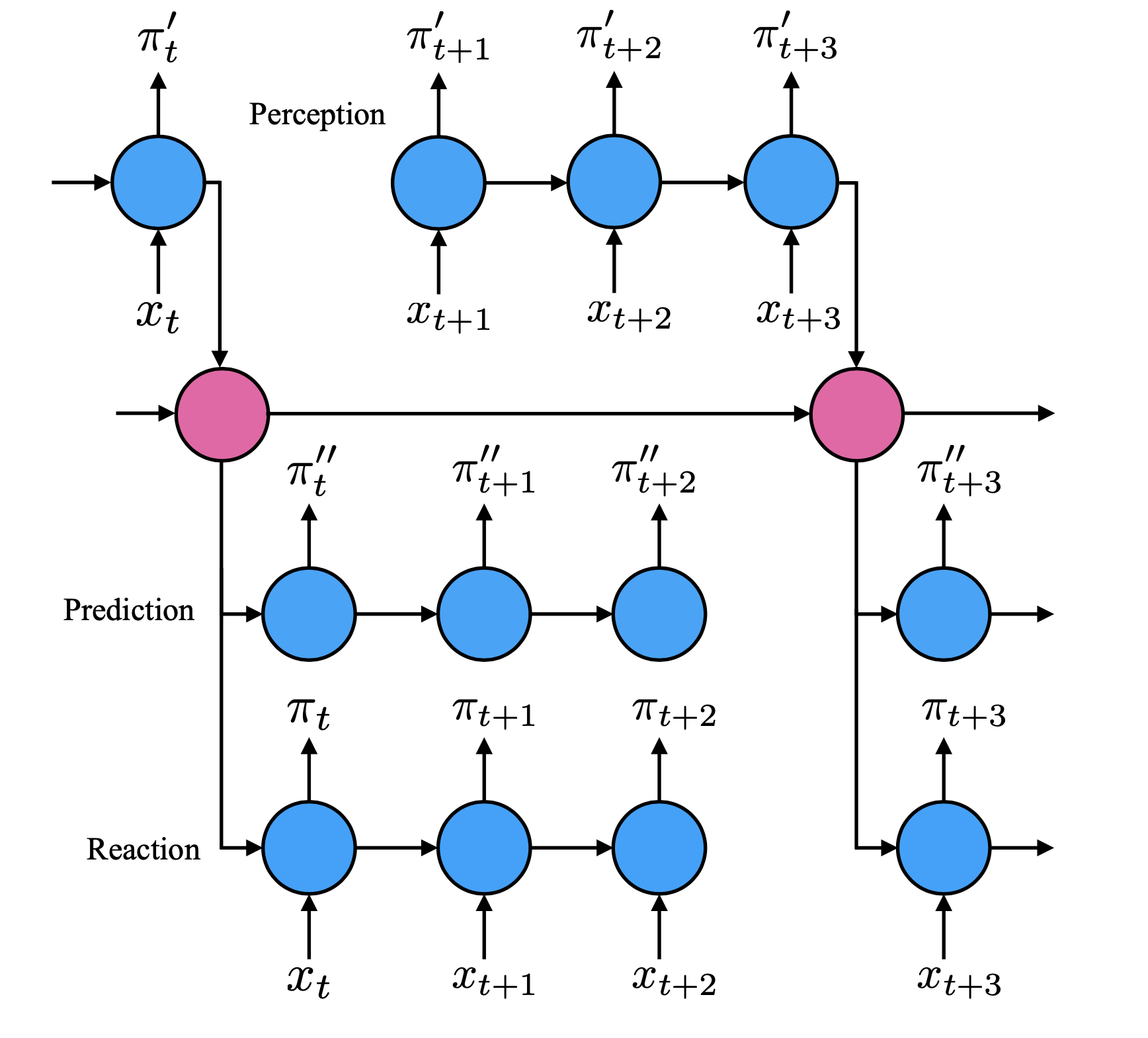
We can even build auxiliary policies to augment the main policy of the agent by leveraging information asymmetry. Stooke et al. proposed a Perception-Prediction-Reaction (PPR) agent by employing a temporal hierarchy and using distances between main and auxiliary policies as a regularization. Concretely, starting from the minimal temporal hierarchy which is essentially two RNNs operating at different time scales to divide and simplify the responsibilities of long-term and short-term memory, PPR utilizes two more fast-ticking RNNs (i.e., operating at the same time scale as the RNN for main policy) with different memory accessibility to create an asymmetry. Specifically, one fast-ticking core is a sensory loop, namely perception, which only takes sensorimotor observations as inputs and outputs to the slow-ticking RNN. Note that it has no access to long-term memory. The other fast-ticking core is a motor loop, namely prediction, which can access the long-term memory but not the observation steams. Its outputs will not go to the slow-ticking RNN either. Finally, the fast-ticking core, Reaction, takes observations and long-term memory as inputs and produces the main policy for the agent. Its outputs will also not go to the slow-ticking core. This architectural design introduces structural priors on the RNN core and creates information asymmetry to regularize both main and auxiliary policies and help to shape the hidden representations. The figure below which is directly from Stooke et al. illustrates this architecture.
Let’s discuss how the auxiliary loss works. In POMDPs, agents can improve their understanding of the current state by incorporating the history of observations and maintaining a hidden state \(h\). It is done in an autoregressive manner with RNN \(h_t=f\left(x_t, h_{t-1}\right)\). Hence, the policy changes from \(\pi\left(a_t \vert s_t\right)\) to \(\pi \left(a_t \vert h_t\right)\). Leveraging temporal hierarchy provided by slow-ticking and fast-ticking cores, i.e., \(h_t^S\) and \(h_t^F\), the policy can handle tasks that require memory ability spanning across longer time axis \(\pi\left(a_t \vert h_t^S, h_t^F\right)\). Following the idea of RL as probabilistic inference and assuming policies as multivariate Gaussian distributions, the main policy from the Reaction branch and auxiliary policies from Perception and Prediction branches can be obtained:
\[\begin{align} &\pi_t = \mathcal{N}\left(\mu_t, \Sigma_t\right) \\ &\pi_t'= \mathcal{N} \left(\mu_t', \Sigma_t'\right) \\ &\pi_t''= \mathcal{N} \left(\mu_t'', \Sigma_t''\right) \\ \end{align},\]where
\[\begin{align} &\mu_t, \Sigma_t = g\left(h_t^{Reaction}\right) \\ &\mu_t', \Sigma_t' = g'\left(h_t^{Perception}\right) \\ &\mu_t'', \Sigma_t'' = g''\left(h_t^{Prediction}\right) \end{align}.\]To encourage each policy to agree as much as possible with other policies despite the different information accessibility, the auxiliary loss contains three KL divergence terms between each two of them:
\[\begin{align} \mathcal{L}_{aux} = \sum_t &D_{KL} \left(\mathcal{N}\left(\mu_t, \Sigma_t \right) \Vert \mathcal{N}\left(\mu_t', \Sigma_t'\right)\right) + \\ &D_{KL} \left(\mathcal{N}\left(\mu_t, \Sigma_t \right) \Vert \mathcal{N}\left(\mu_t'', \Sigma_t''\right)\right) + \\ &D_{KL} \left(\mathcal{N}\left(\mu_t', \Sigma_t' \right) \Vert \mathcal{N}\left(\mu_t'', \Sigma_t''\right)\right). \end{align}\]Intuitively, this auxiliary loss puts two priors on the main policy. Despite the information asymmetry, the main policy should be inferable from an auxiliary policy that only incorporates recent sensorimotor steams, i.e., policy from perception. It also should be expressible from a policy that only accesses long-term memory and cannot access any instant observations, i.e., policy from prediction.
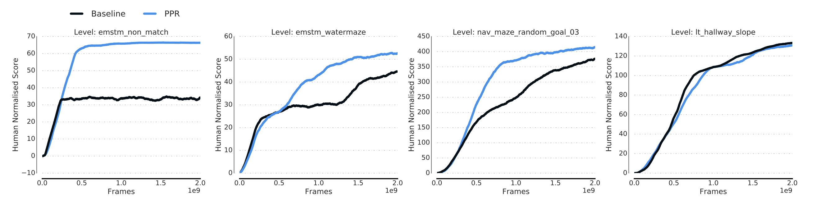
The above experiment results are from Stooke et al., where the PPR agent is compared with a baseline IMPALA agent. We can see that in memory-based levels such as Select Non-matching Object, Watermaze, and Navmaze, the PPR agent significantly outperforms the baseline agent which only utilizes one recurrent module to deal with long-term memory, suggesting the extra auxiliary policies and loss improve the memory ability of the agent. In reactive levels such as Laser tag, the PPR agent does not show any degradation given that the policy becomes less dynamic because it is trained to be easier to be predicted.
Summary
In this post, we have reviewed plenty of auxiliary tasks used commonly in RL. We have familiarized ourselves with their concepts, known how they work, investigated improvements they bring, and examined how they are implemented. Despite their name “auxiliary” which means “supplementary “ — which means the optimization is still dominated by the RL objective — it also means “offering or providing help” — because they do improve the sample efficiency and speed up the learning in many tasks. I sincerely hope that this post can help you understand better if you are not very familiar with them or assist your work through the demo code snippets. Please feel free to raise any questions or point out any errors or mistakes. Lastly, thanks for your interest and reading, and please stay tuned for further posts.